
Reference: Pixabay
데이터사이언스 대학원 강화학습 수업을 듣고 정리한 내용입니다.
John이라는 외국인이 카지도 슬롯머신(한국에서는 사적으로 하면 불법이지만, 일본에서는 길거리에 빠칭코 가게들이 많다)에 들어가서 슬롯 머신으로 게임을 진행하려고 한다. 수 많은 슬롯 머신 기기들이 있는데 어떤 기기에서 칩을 벌 수 있는 확률이 높을까?
Multi-armed Bandits 은 이러한 여러 대(multi)의 레버(armed)를 가진 슬롯 머신(bandits)를 이야기한다. 이 문제는 State 간에 전환(transit)이 없기 때문에 Reinforcement Learning의 제일 간단한 상황이다.
K-armed Bandit Problem

Reference: Pixabay 만약 여러분이 친구랑 두 개의 코인(확률이 공정하고 0.5가 아님)을 가지고 내기를 하는데, 여러분이 선택한 코인이 윗면(head)이 나오면 1를 친구가 가져간다.
이러한 문제를 K-armed bandit 문제라고 한다. 여기서 K는 두 개의 코인 중 선택 해야하는 행동, armed bandit는 코인의 앞면, 뒷면이 나올 수 있는 상황이다.
Formal한 정의를 하자면, 각 time-step 에서 개 행동(Actions)중에 선택된 행동을 라고 하며, 선택에 따라서 기대되는(혹은 평균) 보상을 라고 한다. 따라서 어떤 행동 의 가치(Value) 는 선택된 행동의 보상 기댓값과 같으며 수식으로 다음과 같다.
다만, 우리는 선택된 행동의 가치는 모른다(만약에 알면 모든 사람은 복권에 당첨되었을 것이다). 따라서 선택한 행동의 가치를 추정해야하며, time-step 에서 선택한 행동 의 **가치 추정값(estimated value of action)**을 라고 한다. 우리의 목적은 가 에 가장 근접하게만 만들면 최적의 결과를 얻을 수 있다.
그렇다면 는 어떻게 계산할 수 있을까? 가장 간단한 방법은 현재까지 실행했던 기록을 가지고 계산하는 sample-average 방법이다.
코인을 선택하는 문제에서 다른 사람들이 던져본 기록이 있다면, 우리는 쉽게 두 코인의 를 계산 할 수 있다.
| 실행 index | :coin: 1 | :coin: 2 |
|---|---|---|
| 1 | T | H |
| 2 | H | T |
| 3 | H | H |
| 4 | T | H |
| 5 | T | H |
| 6 | T | T |
Exploitation vs. Exploration
**활용(Exploitation)**과 **탐색(Exploration)**은 강화학습에서 자주 이야기하는 키워드다. 활용(Exploitation)은 현재 주어진 정보를 가지고 최대의 효용을 취하는 것이며 **최적화(Optimization)**과 연관이 있다. 반면 탐색(Exploration)은 미래의 더 높은 효용(Reward)을 얻기위해 정보를 더 취득하는 과정이며 **학습(Learning)**과 연관이 있다.
Epsilon-Greedy
행동의 선택 또한 다양한 방법들이 있는데, 제일 간단한 방법은 탐욕적인(Greedy) 방법이다. 현재 주어진 정보에서 최적의 행동만 선택하는 방법이며 수식으로 다음과 같다.
-Greedy는 의 확률로 탐색(랜덤으로 행동 선택)을 하고, 확률로 활용(최적의 행동 선택)한다.
10-armed Testbed

Figure 1: 10-armed Testbed
“code for Figure 1”
import numpy as np
import matplotlib.pyplot as plt
import seaborn as sns
from tqdm import tqdm
import pandas as pd

plt.style.use('ggplot')
np.random.seed(1234)
k = 10  # number of arms
q_true = np.random.randn(k)

fig, ax = plt.subplots(1, 1, figsize=(8, 4), dpi=1200)
sns.violinplot(data=np.random.randn(1000, 10) + q_true, linewidth=0.8, ax=ax)
ax.set_xlabel("Action")
ax.set_ylabel("Reward distribution")
plt.show()
위 그림과 같이 각 Action()에 해당하는 평균 다르고, 분산이 인 실제 가치 분포가 있다. 이러한 보상을 probabilistic reward라고 한다. 만약에 우리가 이 분포를 알고 있고 계속 10개의 슬롯머신을 돌린다는 상황에서 최적의 선택은 당연히 2번 슬롯일 것이다(평균적으로 기댓값이 높기 때문에).
Sample average 방법으로 각기 다른 을 취해서 최적의 전략(policy)을 찾아보자. 일부 코드는 ShangtongZhang - reinforcement-learning-an-introduction를 많이 참고하였다. 한 번의 실험 run이라고 부르고, 한 번의 run에서 bandit(즉, )을 새로 세팅하고 만큼 k-armed bandit을 경험해 볼 수 있다.
“code for Bandit, simulate and figures”
k = 10
n_run = 2000
n_time = 1000
epsilons = [0, 0.1, 0.01]
bandits = [Bandit(k=k, epsilon=eps, sample_average=True) for eps in epsilons]
rewards, best_action_counts, best_actions = simulate(n_run, n_time, bandits, rt_raw=True)

cols = [f'$\epsilon={eps:.2f}$' for eps in epsilons]
fig, ax = plt.subplots(1, 1, figsize=(8, 4), dpi=1200)
sns.histplot(
    data=pd.DataFrame(best_actions.T, columns=cols),
    bins=10, common_bins=True, discrete=True, multiple='fill', ax=ax)
ax.set_xticks(np.arange(k))
ax.set_xticklabels([f'{i}' for i in range(k)])
ax.set_ylabel('Percentage of best action')
ax.set_xlabel('Actions')
plt.show()

fig, axes = plt.subplots(1, 2, figsize=(16, 4), dpi=1200)
ax1, ax2 = axes
sns.lineplot(data=pd.DataFrame(rewards.T, columns=cols), dashes=False, ax=ax1)
sns.lineplot(data=pd.DataFrame(best_action_counts.T, columns=cols), dashes=False, ax=ax2)
ax1.set_xlabel('Steps')
ax1.set_ylabel('Average reward')
ax2.set_xlabel('Steps')
ax2.set_ylabel('Percentage of Optimal action')
ax1.legend()
ax2.legend()
plt.tight_layout()
plt.show()
class Bandit:
def __init__(
self,
k: int=10,
epsilon: float=0.0,
initial: float=0.0,
true_reward: float=0.0,
step_size: float=0.1,
sample_average: bool=False,
ucb_param: float|None=None,
gradient: bool=False,
gradient_baseline: bool=False,
):
self.k = k
self.actions = np.arange(self.k)
self.epsilon = epsilon
self.initial = initial
self.true_reward = true_reward
self.step_size = step_size
self.average_reward = 0.0
self.sample_average = sample_average
self.ucb_param = ucb_param
self.gradient = gradient
self.gradient_baseline = gradient_baseline
def reset(self):
# real reward for each action at time t
self.q_true = np.random.randn(self.k) + self.true_reward
# estimation for each action at time t
self.q_estimation = np.zeros(self.k) + self.initial
# # of chosen times for each action
self.action_count = np.zeros(self.k)
self.best_action = np.argmax(self.q_true)
self.time = 0
def act(self):
if np.random.rand() < self.epsilon:
return np.random.choice(self.actions)
q_best = np.max(self.q_estimation)
return np.random.choice(np.where(self.q_estimation == q_best)[0])
def step(self, action):
# give reward at time t by choosing action
reward = np.random.randn() + self.q_true[action]
# update records
self.time += 1
self.action_count[action] += 1
self.average_reward += (reward - self.average_reward) / self.time
if self.sample_average:
# update estimation using sample averages
self.q_estimation[action] += (reward - self.q_estimation[action]) / self.action_count[action]
else:
# update estimation with constant step size
self.q_estimation[action] += self.step_size * (reward - self.q_estimation[action])
return rewarddef simulate(n_run: int, n_time: int, bandits: list[Bandit]):
"""Simulate multi-armed bandit experiment
Args:
n_run (int): number of run, each run means using a k-armed bandit with n_times
n_time (int): number of time to experience for each bandit
bandits (list[Bandit]): bandits list, each bandit has different experiment settings
"""
rewards = np.zeros((len(bandits), n_run, n_time))
best_action_counts = np.zeros(rewards.shape)
best_actions = np.zeros((len(bandits), n_run))
for i, bandit in enumerate(bandits):
for r in tqdm(range(n_run), total=n_run, desc=f'Simulating Exp-{i}'):
bandit.reset() # reset bandit: the same bandit can be used for multiple runs
best_actions[i, r] = bandit.best_action
for t in range(n_time):
action = bandit.act()
reward = bandit.step(action)
rewards[i, r, t] = reward
if action == bandit.best_action:
best_action_counts[i, r, t] = 1
mean_best_action_counts = best_action_counts.mean(axis=1)
mean_rewards = rewards.mean(axis=1)
return mean_rewards, mean_best_action_counts, best_actions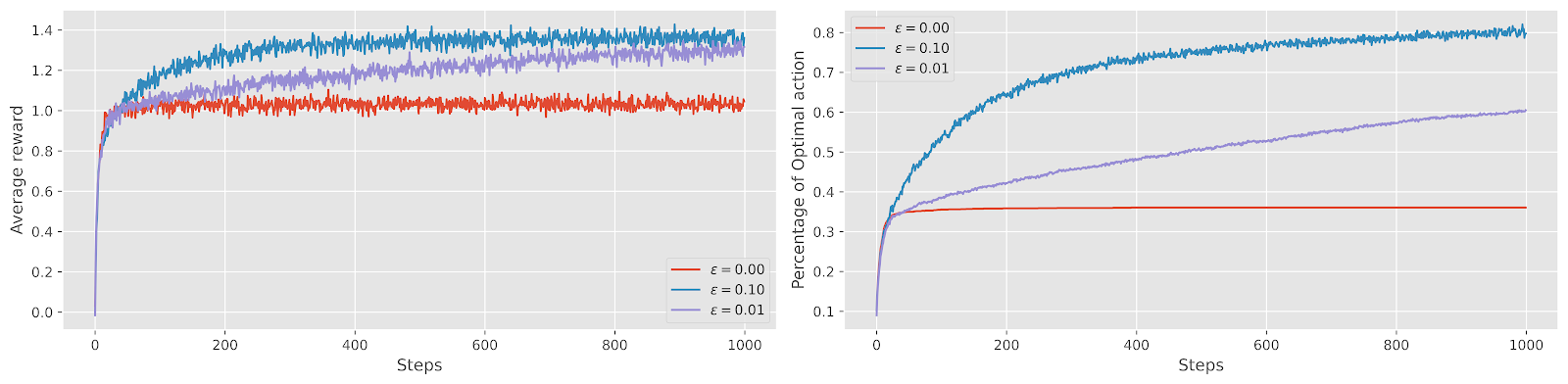
Figure: epsilon greedy
실험 결과 초깃값이 모두 동일()할 때, greey policy는 평균적으로 의 보상을 얻었다. 이 높을 수록 탐색 초기에는 보상이 높았으나, 시간이 점점 지날 수록 작은 과 큰 간의 간극이 줄어든 것을 볼 수 있다. 다만, 최적의 선택을 고른 비율에서는 탐색을 상대적으로 많이 하는 경우 경험을 많이 할 수록 더 높다는 것을 알 수 있다. 높은 의 문제점은 최적의 선택이 어떤 것인지 대략 안 상황에서 계속해서 10% 확률로 다른 것을 탐색한 다는 것이다. 즉, 효율적이지 않다는 것이다.

행여나 실험에서 Best Action이 불균형하게 세팅될 수도 있다는 걱정이 있었는데, 각 실험 Bandit의 best action histogram을 그려보니, 모든 action이 거의 균등하게 세팅되어 있었다(3개 실험의 bar의 길이가 비슷비슷하다).
만약에 보상에 더 많은 노이즈(noise)가 있다고 하면, greedy 보다 -greedy가 더 좋은 전략이 될 수 있을까? 물론 그렇다, 더 많은 탐색을 할 수록 더 높은 보상을 취할 수 있을 것이다. 이런 점이 탐색(exploration)을 **“학습한다”**라고 말하는 이유다. 그렇다면 determinsitic reward이면 어떻게 될까? 이때 최적의 전략은 각 action을 한 번씩 취한 다음에 greedy 전략으로 가는 것이다.
Incremental Implementation
기존의 sample average 방법은 간단하지만, 모든 선택을 저장해야 된다는 단점이 있다(공간 복잡도: ). 아래와 같은 방법으로 공간복잡도를 로 해결 할 수 있다.
Step Size and Convergence
Incremental update에서 은 step size(혹은 Learning Rate)라고 하는데, 이를 함수 로 치환 할 수 있다. 단, 수렴(convergenence)해야하는 제약 조건이 있다.
Optimistic Initial Values
초깃값도 최적의 선택에 영향을 준다. 아래 그림에서 greedy 전략은 초깃값이 5이지만 초깃값이 0인 -greedy 전략보다 더 낮은 보상을 얻었다.

UCB Action Selection
행동 선택시 고정된 특정 확률로 선택하는 것이 아니라 보상 upper-bound가 높은 행동을 선택하면 더 좋지 않을까? Upper-Confidence-Bound (UCB) 알고리즘은 이러한 점을 반영한다. 는 행동이 선택된 횟수, 는 탐색의 정도를 조절한다.
def act(self):
    # ...
    if self.ucb_params is not None:
        # A_t = arg max_a ( Q_t + c * sqrt(ln(t) / n) )
        ucb_estimation = self.q_estimation + \
            self.ucb_params * np.sqrt(np.log(self.time + 1) / (self.action_count + 1e-5))
        q_best = np.max(ucb_estimation)
        return np.random.choice(np.where(ucb_estimation == q_best)[0])
    # ...
“code for figures”
fig, axes = plt.subplots(1, 2, figsize=(16, 4), dpi=1200)
cols = [f'$\epsilon={eps:.2f}, ucb={ucb_param}$' for (eps, ucb_param) in zip(epsilons, ucb_params)]
ax1, ax2 = axes
sns.lineplot(data=pd.DataFrame(rewards.T, columns=cols), dashes=False, ax=ax1)
sns.lineplot(data=pd.DataFrame(best_action_counts.T, columns=cols), dashes=False, ax=ax2)
ax1.set_xlabel('Steps')
ax1.set_ylabel('Average reward')
ax2.set_xlabel('Steps')
ax2.set_ylabel('Percentage of Optimal action')
ax1.legend()
ax2.legend()
plt.tight_layout()
plt.show()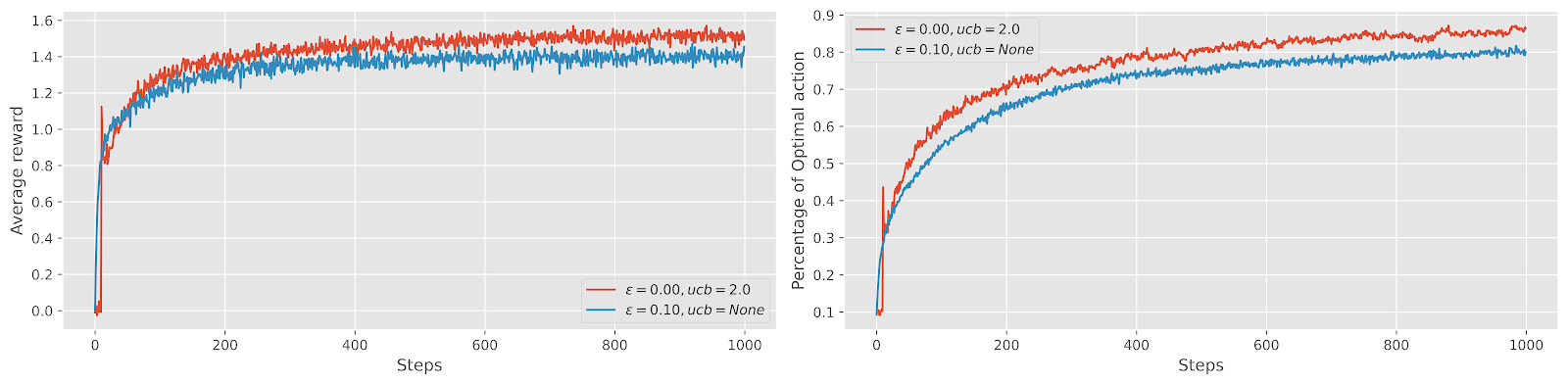
시뮬레이션 결과 UCB를 사용한 greedy 전략이 UCB를 사용하지 않은 -greedy 전략 보다 더 높은 평균 보상을 획득했다.
일때의 를 보면 다음과 같다. 선택된 actions 횟수를 다음과 같은 테이블에 정리해뒀다. 아래 그림을 보면 탐색을 많이 한 3번 action에 대해서 upper bound가 많이 줄어든 모습을 볼 수 있다. 즉, 점점 해당 선택에 대한 불확실성이 줄어들었다고 볼 수 있다.
| action | 0 | 1 | 2 | 3 | 4 | 5 | 6 | 7 | 8 | 9 |
|---|---|---|---|---|---|---|---|---|---|---|
| count | 6 | 2 | 5 | 842 | 71 | 5 | 6 | 5 | 55 | 3 |
 |
Gradient Bandit Algorithms
Gradient Bandit 알고리즘은 각 행동에 대한 선호도 를 학습하는 하는 방법이다. 큰 선호도를 가지면 더 자주 선택되며, 보상과는 전혀 상관성이 없다. 그 중 하나로, Soft-max (Boltzmann) distribution 방법이 있다. 수식을 보면 사실상 보상을 확률화해서 반영한 알고리즘이다.
행동 을 선택하고 보상 을 받으면 그때 선호도를 업데이트 한다. 는 시점 이전의 평균 보상값, 는 step size다.
def act(self):
    # ...
    if self.gradient:
        exp_estimation = np.exp(self.q_estimation)
        self.action_prob = exp_estimation / exp_estimation.sum()
        return np.random.choice(self.actions, p=self.action_prob)
# ...def step(self):
# ...
elif self.gradient:
one_hot = np.zeros(self.k)
one_hot[action] = 1
if self.gradient_baseline:
baseline = self.average_reward
else:
baseline = 0
self.q_estimation += self.step_size * (reward - baseline) * (one_hot - self.action_prob)
# ...
“code for figures”
# np.random.seed(1234)
k = 10
n_run = 2000
n_time = 1000
step_sizes = [0.1, 0.1, 0.4, 0.4]
gradient_baselines = [True, False, True, False]
bandits = [
    Bandit(k=k, gradient=True, step_size=step_size, gradient_baseline=gradient_baseline, true_reward=4)
    for (step_size, gradient_baseline) in zip(step_sizes, gradient_baselines)
]
rewards, best_action_counts, best_actions = simulate(n_run, n_time, bandits)

fig, axes = plt.subplots(1, 2, figsize=(16, 4), dpi=1200)
cols = [f'$\\alpha={step_size:.2f}, baseline={gradient_baseline}$'
        for (step_size, gradient_baseline) in zip(step_sizes, gradient_baselines)]
ax1, ax2 = axes
sns.lineplot(data=pd.DataFrame(rewards.T, columns=cols), dashes=False, ax=ax1)
sns.lineplot(data=pd.DataFrame(best_action_counts.T, columns=cols), dashes=False, ax=ax2)
ax1.set_xlabel('Steps')
ax1.set_ylabel('Average reward')
ax2.set_xlabel('Steps')
ax2.set_ylabel('Percentage of Optimal action')
ax1.legend()
ax2.legend()
plt.tight_layout()
plt.show()
Baseline은 의 사용 여부다. 큰 step size를 사용할 수록 초기에는 탐색을 하여 빠른 최적의 선택을 할 수 있지만, 작은 step size와 를 사용하여 느리지만 더 많은 최적의 선택을 할 수 있게 만들 수 있다.
Non-stationary Rewards
Stationary reward란 시간이 지나도 보상의 변동이 일정한 것(혹은 분포가 일정)을 말한다. 이때 step size는 보통 시간에 따라서 작아진다.
Non-stationary reward는 시간에 따라서 보상의 변동이 일정하지 않은 것(혹은 분포가 달라짐)을 말한다. 이때 step size는 보통 일정한 값을 사용한다.