데이터사이언스 대학원 강화학습 수업을 듣고 정리한 내용입니다.
Policy Evaluation & Policy Improvement
The term dynamic programming (DP) refers to a collection of algorithms that can be used to compute optimal policies given a perfect model of the environment as a Markov decision process (MDP)
강화학습에서 우리가 완전한 dynamic을 알고 있을 때, DP로 다음 문제를 해결하기 위해 사용한다.
- Policy Evaluation(prediction problem): 주어진 policy에서 value fuction을 반복적으로 연산하는 과정(MDP, )
- Policy Improvement(control): value function이 주어졌을 때, 향상된 policy를 계산하는 것(MDP, )
Policy Evaluation
Policy Evaluation은 policy 가 주어졌을 때, Value function 를 계산한다. Policy Evaluation Update Rule은 다음과 같으며, 여기서 는 번째 policy다.
Example: 4 x 4 Grid-World

이번 Grid-World 예시는 다음과 같다.
* Non-terminal states $S = \lbrace 1, 2, \cdots, 14 \rbrace$, 회색 영역은 terminal state.
* State Transition($s \rightarrow s'$)은 $-1$의 보상을 얻고, grid밖을 벗어나면 이전 state에 있는 것으로 간주한다. 즉, 많이 움직일 수록 안좋다.
* Actions $\mathcal{A} = \lbrace \uparrow, \downarrow, \rightarrow, \leftarrow \rbrace$
* Uniformly random policy $\pi(a \vert s) = 0.25$ for all $a \in \mathcal{A}$ and for all non-terminal states $s \in \mathcal{S}$
* Deterministic state transition & reward model $p(s', r \vert s, a)$
    * 예시1: $p(s'=6, r=-1 \vert s=5, a=\rightarrow)=1$, grid 5에서 우측 행동($\rightarrow$) 선택 시 grid 6으로 가고 보상도 $-1$을 얻을 확률은 1.
    * 예시2: $p(s'=7, r=-1 \vert s=7, a=\rightarrow)=1$, grid 7에서 우측 행동($\rightarrow$) 선택 시 grid 7으로 가고 보상도 $-1$을 얻을 확률은 1.
    * 예시3: $p(s'=10, r=r' \vert s=5, a=\rightarrow)=0 \ \forall r' \in \mathcal{R}$, grid 5에서 우측 행동($\rightarrow$) 선택 시 grid 10으로 갈 수 있는 확률은 0.
* $\gamma=1.0$를 가정한다.
그렇다면 이러한 MDP 환경에서 최대의 보상은 무엇일까? 당연히 제일 적은 스텝으로 terminal state에 도달하는 것이다.
따라서 Initial State 를 만들고 계속해서 policy evaluation을 진행해보자. 메모리에 상관없이 각 좌표에서 replace하지 않고 두 개의 matrix로 업데이트 한다고 가정한다.
| (i, j) | 0 | 1 | 2 | 3 |
|:-:|:-:|:-:|:-:|:-:|
| 0 | 0.0 | 0.0 | 0.0 | 0.0 |
| 1 | 0.0 | 0.0 | 0.0 | 0.0 |
| 2 | 0.0 | 0.0 | 0.0 | 0.0 |
| 3 | 0.0 | 0.0 | 0.0 | 0.0 |

초기 상태 가치는 모두 0.0이다.| (i, j) | 0 | 1 | 2 | 3 |
|:-:|:-:|:-:|:-:|:-:|
| 0 | 0.0 | -1.0 | -1.0 | -1.0 |
| 1 | -1.0 | -1.0 | -1.0 | -1.0 |
| 2 | -1.0 | -1.0 | -1.0 | -1.0 |
| 3 | -1.0 | -1.0 | -1.0 | 0.0 |
각 state $s \in \mathcal{S}$ 에서 Bellman equation을 사용하여 업데이트 하면 위의 표와 같다.예를 들어, 좌표 `(0, 2)` $s=2$에서 $s' \in \lbrace 1, 2, 3, 6 \rbrace$의 transition을 제외하고 모두 확률이 0이 되기 때문에 다음과 같이 $v_{k+1}(s)$를 계산할 수 있다.다른 예시로 terminal state 중 하나인 좌표 `(0, 0)`은 모든 transition에 대하여 확률이 0이기 때문에 계속 $0.0$ 이다. | (i, j) | 0 | 1 | 2 | 3 |
|:-:|:-:|:-:|:-:|:-:|
| 0 | 0.0 | -1.75 | -2.0 | -2.0 |
| 1 | -1.75 | -2.0 | -2.0 | -2.0 |
| 2 | -2.0 | -2.0 | -2.0 | -1.75 |
| 3 | -2.0 | -2.0 | -1.75 | 0.0 |
각 state $s \in \mathcal{S}$ 에서 Bellman equation을 사용하여 업데이트 하면 위의 표와 같다.예를 들어, 좌표 `(1, 2)` $s=6$에서 $s' \in \lbrace 5, 2, 7, 10 \rbrace$를 제외하고 모두 확률이 0이 되기 때문에 다음과 같이 $v_{k+1}(s)$를 계산할 수 있다.다른 예시로, 좌표 `(0, 1)` $s=1$에서 $s' \in \lbrace \text{terminate}, 1, 2, 5 \rbrace$를 제외하고 모두 확률이 0이 되기 때문에 다음과 같이 $v_{k+1}(s)$를 계산할 수 있다.## Policy ImprovementPolicy Improvement는 value function 가 주어졌을 때, 향상된 policy 을 구하는 것이다.
Let $\pi$ and $\pi'$ be any pair of deterministic policies such that, for all $s \in \mathcal{S}$, $q_{\pi}\big(s, \pi'(s) \big) \geq v_{\pi}(s)$.

Then the policy $\pi'$ must be as good as, or better than $\pi$.
Theorm을 풀어 쓰자면, 새로운 policy 에서의 action-value가 state-value 보다 같거나 높다면, 는 보다 같거나 좋은 policy다. 따라서 improved policy 를 얻기 위해서는 action-value function을 최대화 하는 policy를 선택하면 된다.
최종적으로 improved policy는 action-value가 최대가 되는 action을 선택하는 policy가 된다. 예: $s=1$에서 improved policy는 $\leftarrow$좌: $v_k$, 우: greedy policy with $v_k$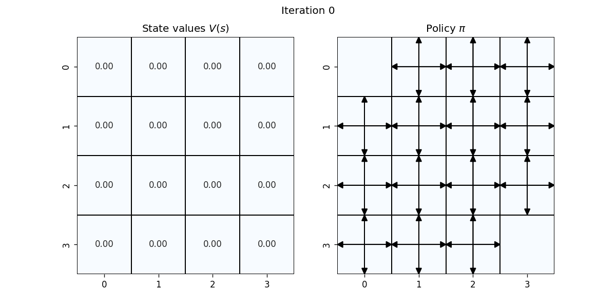
좌: $v_k$, 우: greedy policy with $v_k$
좌: $v_k$, 우: greedy policy with $v_k$
좌: $v_k$, 우: greedy policy with $v_k$
좌: $v_k$, 우: greedy policy with $v_k$
좌: $v_k$, 우: greedy policy with $v_k$
Policy Iteration
우리의 최종 목적은 결국 최적의 policy를 구하는 것이다. Policy Iteration은 policy evaluation()과 improvement()를 반복하는 과정이다.

2. Policy Evaluation

    - $\Delta$: 이전의 value와 현재 value의 차이
    - $v$: 이전 value 저장
    - 모든 state $s$ 에서 벨만 업데이트를 통해 현재 $s$의 value $V(s)$를 구한다.
    - $v$와 $V(s)$의 차이 절댓값과 $\Delta$중 큰 것을 남긴다.
    - $\Delta$가 아주 작은 임의의 수 $\theta$보다 작을 때 까지 Policy Evaluation을 한다.

3. Policy Improvement

    - 모든 state $s$ 에서 value가 가장 큰 action을 선택하여 policy $\pi(s)$ 로 지정
    - `old-action` 이 현재 policy $\pi(s)$와 같이 않으면 아직 `policy-stable` 상태가 아닌 것이다.
    - `policy-stable` 상태면 멈추고 최적의 value $v_*$와 최적의 policy $\pi_*$ 반환
Value Iteration
Policy Iteration의 단점은 매 스텝마다 policy evaluation이 포함된다는 것이다. 한번에 가능하게 만들 수 없을까?

Generalized Policy Iteration

the general idea of letting policy-evaluation and policyimprovement processes interact, independent of the granularity and other details of the two processes
Policy evaluation과 policy imporvement의 반복이라 볼 수 있다. 그리고 매 스텝마다 최적만 찾을 필요는 없다. approximate policy and approximate value function를 통해서 적당히 좋은 최적값을 찾으면 최종적으로 최적의 값을 찾게 된다.